Theory
Waiting Times and Memory
A single cell spends a stochastic amount of time to execute a division, death or differentiation event – the so-called waiting time \(\tau\). The distribution of waiting times in cell populations, as an ensemble of many single-cell fates, hence quantifies the probabilistic dynamics of basic cellular decisions. Subsequently, we will outline the theoretical concepts employed in MemoCell to describe and infer stochastic processes of multiple possibly interlinked waiting time distributions.
We introduce waiting time distributions from the “view” of a single cell executing a single reaction (e.g., a differentiation event). The next section then generalises the concepts for an ensemble of cells, also being subject to cellular pathways of multiple reactions.
The most basic waiting time distribution is the exponential distribution (see Figure below); \(\tau \sim \mathrm{Exp}(\theta)\) where \(\theta\) is the rate parameter. The mean waiting time is the inverse of the rate, \(\mathrm{E}(\tau)=1/\theta\), and the variance is \(\mathrm{Var}(\tau)=1/\theta^2\). This also implies that the variability of exponential waiting times is always fixed, as measured by the coefficient of variation; \(\mathrm{CV}(\tau)=\frac{\sqrt{\mathrm{Var}(\tau)}}{\mathrm{E}(\tau)} = 1\).

The exponential distribution is the only continuous distribution that fulfils the property of memorylessness, meaning \(p(\tau > t + s | \tau > s) = p(\tau > t)\). This is also why stochastic processes that fulfil the Markov property of memorylessness are characterised by exponential waiting times for their single transition events. Markov jump processes with exponential waiting times allow powerful analytical access [3]. However, the exponential waiting time distribution in itself is often not a good assumption for biological transitions. Applied to cell division, one would assume that the next division event is most likely to occur immediately after the previous division (the mode is at 0); contradicting the fact that cells need a minimal time span to replicate the DNA etc.
For this reason MemoCell allows to describe and infer more general, non-exponential waiting time distributions – specifically the Erlang and phase-type distributions. Indeed, phase-type distributions are “dense” (in the mathematical sense) in the field of all positive-valued distributions; as such, they can approximate any waiting time distribution arbitrarily closely [2] [13]. Importantly, these distributions can be constructed by transitions over multiple states in Markov jump processes (i.e., as convolutions or mixtures of exponential distributions) [2] [4] [9] and thus we retain the analytical tractability.
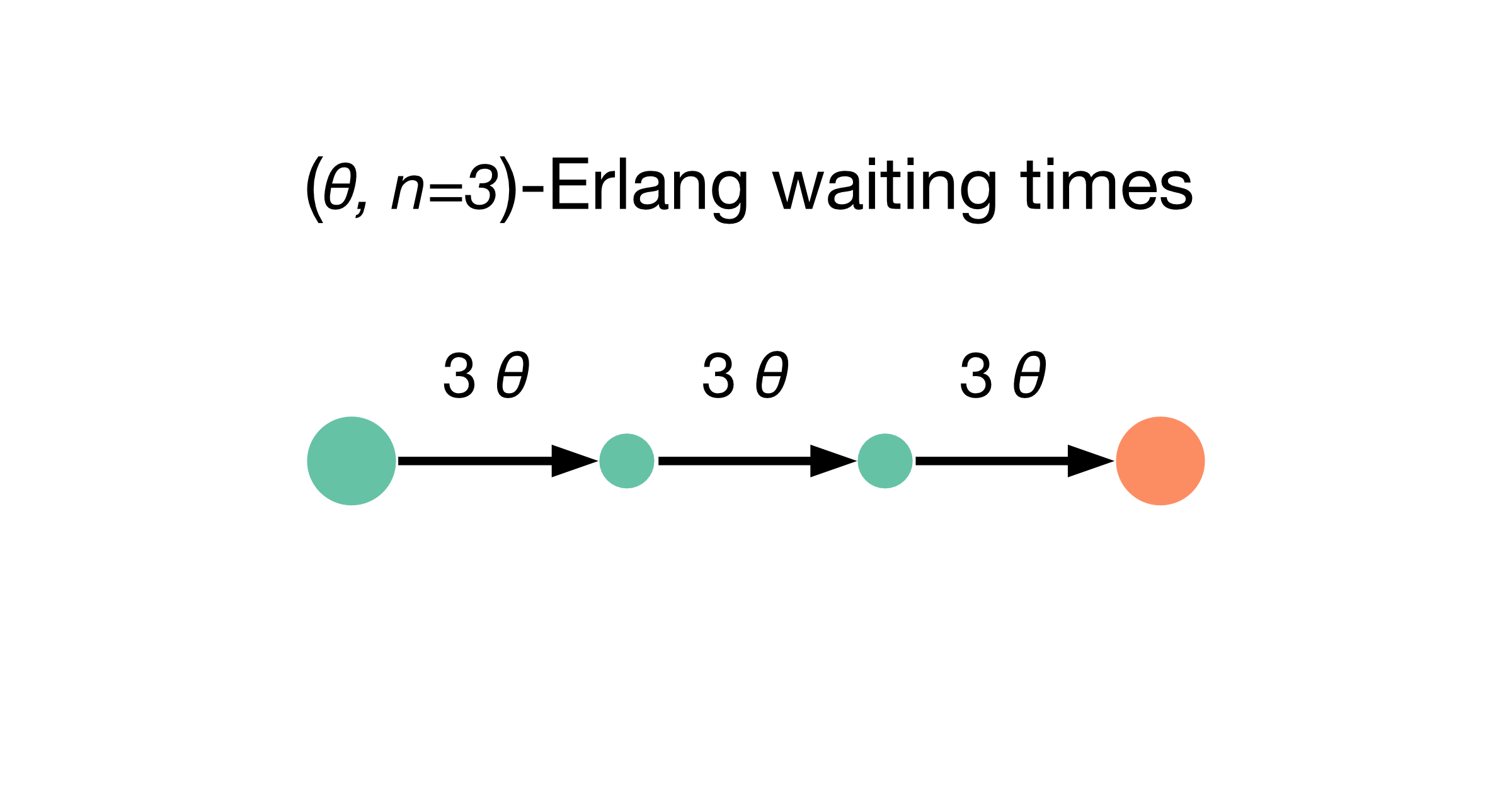
This principle is demonstrated best with the Erlang distribution. An Erlang waiting time \(\tau\) is generated when a single cell passes through a sequence of \(n\) (fictitious, hidden) states, each with independent and identically distributed exponential waiting times \(\tau_i\), \(i=(1,...,n)\) [5]. In MemoCell we parametrise \(\tau_i \sim \mathrm{Exp}(n \theta)\); then \(\tau = \sum_i \tau_i \sim \mathrm{Erl}(n,n\theta)\) is Erlang distributed with mean \(\mathrm{E}(\tau)=1/\theta\) and variance \(\mathrm{Var}(\tau)=1/(n \theta^2)\). The Figure below illustrates the transition graph for such an \((\theta, n=3)\)-Erlang waiting time (to reach the orange state, starting at the leftmost green state).
High number of steps \(n\) can decrease the variability of the distribution as \(\mathrm{CV}(\tau)=1/\sqrt{n}\) (see Figure below, same mean for all cases). The exponential distribution is the special case of the Erlang distribution for \(n=1\). (For a given number of the hidden states the Erlang distribution is actually the phase-type distribution with the lowest variability [1] [12]).

Next to the direct description of the waiting times as done above, a second equivalent description is obtained via the master equation characterising the Markov process on the level of the (hidden) states [the master equation is also known as Kolmogorov forward (and backward) equation; sometimes in slightly different notation].
For the \(n=3\) example, a single cell is either in one of the three “green” states \(w_1=(1,0,0,0)\), \(w_2=(0,1,0,0)\), \(w_3=(0,0,1,0)\) or in the “orange” state \(w_\infty=(0,0,0,1)\). The orange state is absorbing, meaning that the process will jump into this state eventually. With the probability row vector \(\pmb{p}(w, t)=\big(p(w_\infty, t), p(w_1, t), p(w_2, t), p(w_3, t) \big)\), the complete probabilistic dynamics are given by the master equation
where
is the generator or transition rate matrix. The master equation is a (here finite, but possibly infinite) system of differential equations, balancing the probability in- and outflux for each state. Note that we can rewrite
where \(\pmb{s}=-S\,\pmb{1}\) with \(\pmb{1}\) a column vector of ones. The submatrix \(S\) is now the generator/transition rate matrix for the transient states (\(w_1, w_2, w_3\)) only.
These considerations motivate phase-type distributions. As before, we describe the waiting time \(\tau\) to reach one absorbing state \(w_\infty\); now however, jumps may occur between \(m\) transient states, connected by an arbitrary transition rate matrix \(S\) (or subgenerator/transient generator).
We derive the phase-type density and distribution function for \(\tau\). The probabilities to be in any specific transient state are denoted by the row vector \(\pmb{p}(w, t) = \big(p(w_1, t), ..., p(w_m, t) \big)\); the probability to be in any one of them at all is their sum, i.e. \(\pmb{p}(w, t) \, \pmb{1}\). Hence we have the following equations
the probability to be not yet in the absorbing state. Again, the dynamics of the state probabilities (transient states only) are given by the master equation \(\partial_t \, \pmb{p}(w, t) = \pmb{p}(w, t) \, S\). This finite system of differential equations has the general solution
where \(\mathrm{exp}\) is the matrix exponential and the row vector \(\pmb{\alpha}=\pmb{p}(w, t_0)\) denotes the initial probabilities of the transient states at \(t_0=0\). The inverse of the survival probability \(p(\tau > t)\) is the waiting time distribution function \(F(t)=p(\tau \le t)=1-p(\tau > t)\) and thus we obtain
which also directly implies the probability density by differentiation
where \(\pmb{s}=-S\,\pmb{1}\) as above. We call \(\tau\) phase-type (PH) distributed with initial probabilities \(\pmb{\alpha}\) and transient generator \(S\). Due to the denseness of phase-type distributions and the fact that they arise naturally as waiting times over transition graphs in analytically tractable Markov processes, they constitute a powerful approach to represent virtually any waiting time distribution. Exponential, Erlang and other distributions are special cases of phase-type distributions. Mean and variance can be computed by \(\mathrm{E}(\tau)=-\pmb{\alpha}S^{-1}\pmb{1}\) and \(\mathrm{Var}(\tau)= 2\pmb{\alpha}S^{-2}\pmb{1}-(\pmb{\alpha}S^{-1}\pmb{1})^2\), respectively. Note that phase-type representations are generally not unique, i.e. multiple transient generators may exists for the same density and distribution function [11].
MemoCell allows to implement any phase-type waiting times (at least theoretically; with the use of simulation_variables). Particularly easy to implement are phase-type distributions of two or more parallel Erlang channels diverging from a common start state (see application in our release paper or Figure below).
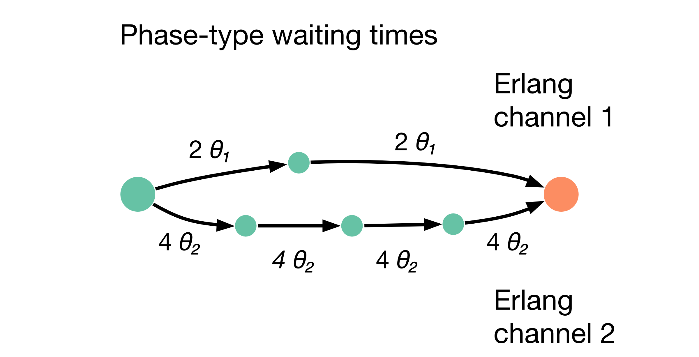
In the Figure example we have used 2-step and 4-step Erlang channels that together construct a quite long-tailed waiting time distribution (Figure below); in comparison the weighted densities of the individual (0.03,4) and (0.04,2) Erlang channels.
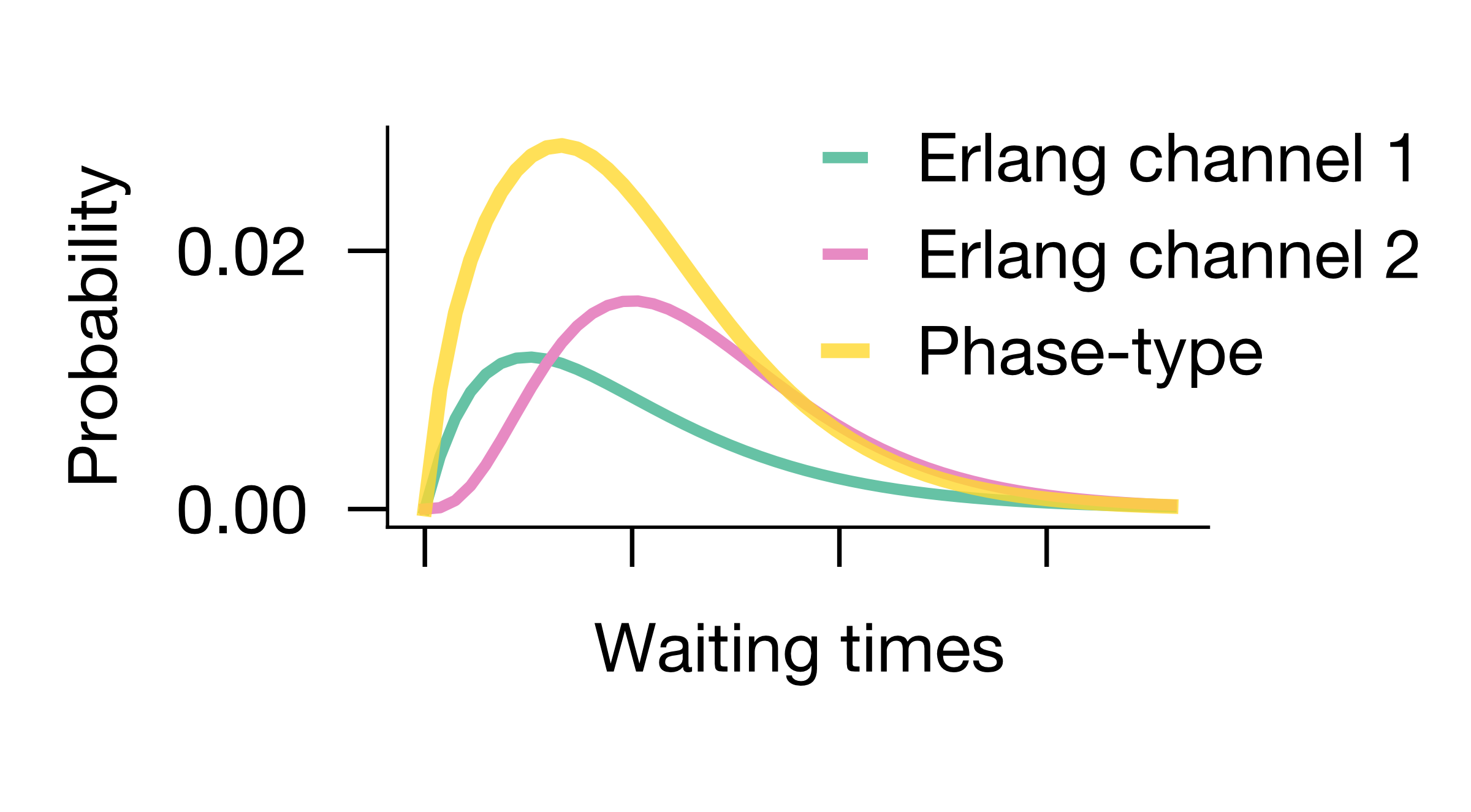
The CV of such phase-type distributions with parallel Erlang channels can be larger or smaller than (or equal to) 1. Note that already finite mixtures of Erlang distributions are dense in the field of positive-valued distributions [2] [13], so we believe that this approach may provide a versatile start point for many problems.
Stochastic Processes
Based on these ideas we now construct a class of (non-Markovian) stochastic processes. Single reactions of phase-type waiting times are now assembled together into multi-reaction networks. Such processes can be implemented in MemoCell and inferred from cell count data.
We introduce a main/observable layer – the dynamics we are interested in – and a hidden layer – which is governed by Markovian dynamics and contains all the fictitious variables and states to construct the more complex waiting times. Different reaction types are available in MemoCell and for each of them the same principle is used to generate Erlang and possibly phase-type waiting times: A reaction is only executed (and seen on the observable layer) via the final jump into the absorbing variable; all the previous jumps between the transient states happen on the hidden layer (and are not seen on the observable layer).
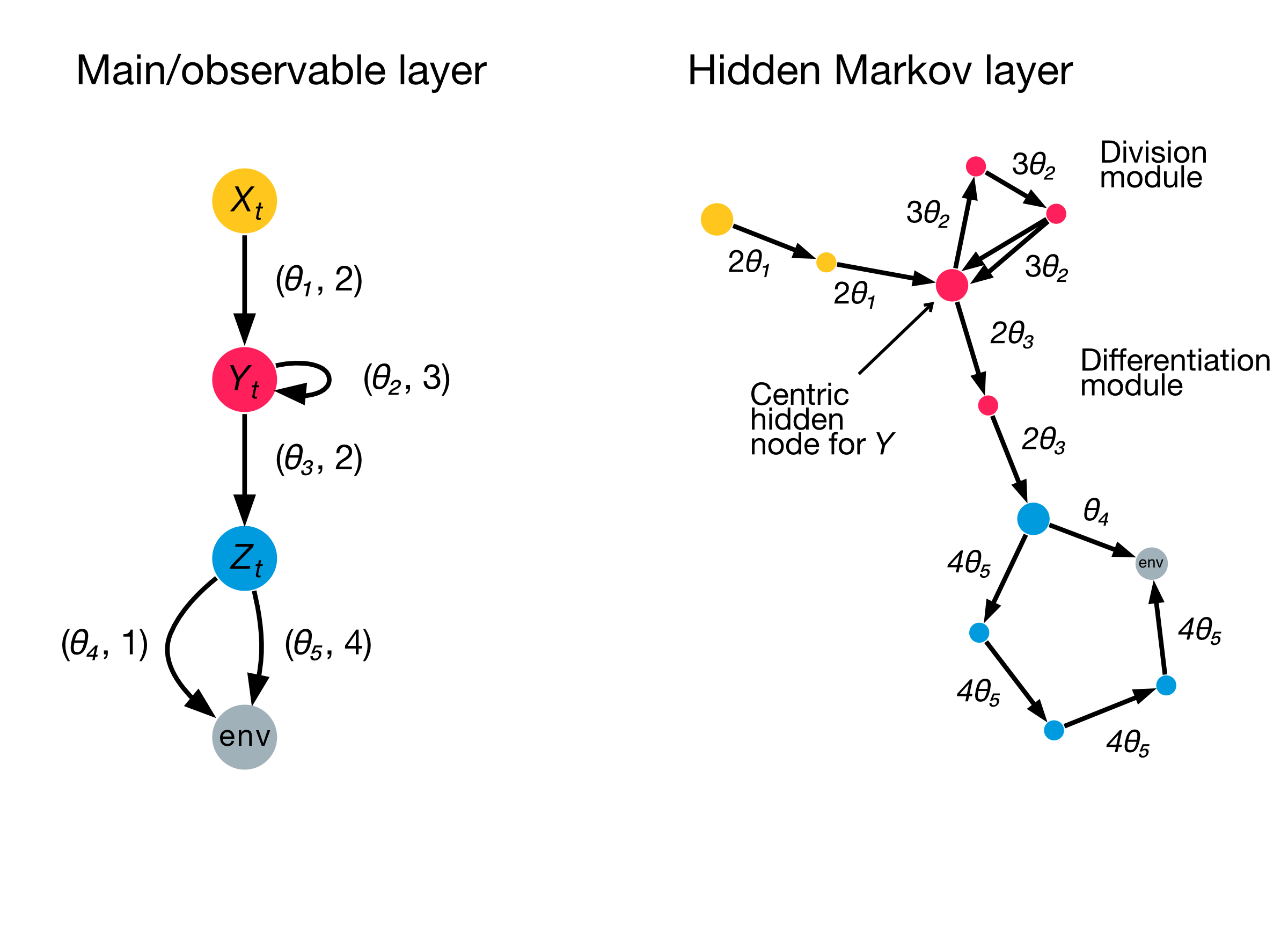
The Figure above gives an example. We have three observable cell types \(X\), \(Y\) and \(Z\), each with cell numbers from \(\{0,1,2,3,...\}\). Cells of \(X\) may differentiate to \(Y\), cells of \(Y\) may differentiate to \(Z\) and also symmetrically divide, cells of \(Z\) leave the system (env is a helper environment variable). The reaction arrows on the main layer are annotated by \((\theta, n)\) tuples, specifying the Erlang channels to generate the reaction waiting times; the hidden Markov layer is populated accordingly with the required number of hidden variables and transitions.
Currently MemoCell offers the following set of zero- and first-order reaction types
\(S \rightarrow E\) (cell differentiation),
\(S \rightarrow S + S\) (symmetric self-renewing division),
\(S \rightarrow S + E\) (asymmetric division),
\(S \rightarrow E + E\) (symmetric differentiating division),
\(S \rightarrow\) (efflux or cell death) and
\(\rightarrow E\) (influx or birth),
where \(S\) is the start cell type and \(E\) is the end cell type. For example, the differentiation reaction from \(X\) (start node) to \(Y\) (end node) was implemented by the type \(S \rightarrow E\); any single cell of cell type \(X\) that undergoes the reaction will switch to cell type \(Y\) at the final (=second) jump of this Erlang channel.
Mathematically, the stochastic process on the observable layer is simply the sum of the Markov processes for the corresponding hidden layer variables. For each cell type \(i \in \{1,...,v\}\), where \(v\) is the total number of cell types, we have a stochastic process for its cell numbers given by
summing all its hidden Markov processes \(W^{(i,j)}_t\); \(u_i\) is the total number of hidden variables of cell type \(i\). In the Figure above we have three cell types with concrete notation \(X_t = W^{(1)}_t\), \(Y_t = W^{(2)}_t\) and \(Z_t = W^{(3)}_t\); and for example \(X_t = W^{(1,1)}_t + W^{(1,2)}_t\) summing the two yellow hidden variables. Technically, this setup allows to encode the hidden layer transitions between the transient states as “differentiation” reactions as the observable cell numbers of the cell type will stay unaltered.
NOTE: These stochastic processes typically live in a countable, but infinite state space and thus cannot be trivially solved through the master equation and the matrix exponential on the hidden layer.
In the previous section, the waiting times were introduced for a single cell passing through the states of a reaction (and in any case, this is what the waiting time and its rate refer to). However this is not limiting: The stochastic processes here readily work for ensemble/population of many single cells placed in the network. If \(w\) cells are available for a transition on the hidden layer, each with a waiting time \(\tau_i \sim \mathrm{Exp}(\lambda)\), the fastest cell will cause the state change. I.e., we look for \(\tau = \mathrm{min}(\tau_1, ..., \tau_w)\) which is distributed as \(\tau \sim \mathrm{Exp}(w \lambda)\). Thus one can upscale the transition rates in the master equation and in simulations to calculate the ensemble-level dynamics.
In this manner, MemoCell offers standard stochastic simulations for the defined class of stochastic processes. A Gillespie algorithm [6] [7] is used on the hidden Markov layer and afterwards the observable layer is obtained by summation.
The second kind of simulations are so-called moment simulations. MemoCell provides the solutions of means, variances and covariances of cell type numbers over time, derived for any user-defined network and parameters. These solutions are exact for the set of available reaction types and relatively fast to compute (compared to stochastic simulations). Thereby they form the basis of the Bayesian inference in MemoCell.
To compute the moments, MemoCell again exploits the analytical access via the Markov jump processes on the hidden layer. The approach of the probability generating function \(G\) is employed, leading to a closed ordinary differential equation system for the first and second (mixed and factorial) moments of the hidden layer variables; for more info, see API docs or the methods of our release paper. MemoCell derives this system symbolically (as an application of sympy and metaprogramming) and integrates it numerically. Concretely one obtains time-dependent \(\mathrm{E}\big(W^{(i,j)}_t\big)\), \(\mathrm{E}\big(W^{(i,j)}_t \, (W^{(i,j)}_t-1)\big)\) and \(\mathrm{E}\big(W^{(i,j)}_t \, W^{(k,l)}_t\big)\) for all hidden variables (where \(i,k \in \{1,...,v\}\), \(i \ne k\), \(j \in \{1,...,u_i\}\), \(l \in \{1,...,u_k\}\)). These hidden layer moments are then automatically added up to obtain the means, variances and covariances on the main/observable layer. First we see that the mean for each cell type \(i\) is given by
the variance for each cell type \(i\) is given by
where \(j,l \in\{1,...,u_i\}\), and the covariance between two different cell types \(i\) and \(k\) is given by
where \(j \in\{1,...,u_i\}\) and \(l \in\{1,...,u_k\}\). Then, the result is obtained by expressing the variances and covariances of the hidden variables in terms of their moments, i.e. using \(\mathrm{Var}(X)=\mathrm{E}(X(X-1))+\mathrm{E}(X)-\mathrm{E}(X)^2\) and \(\mathrm{Cov}(X, Y)=\mathrm{E}(X Y)-\mathrm{E}(X) \mathrm{E}(Y)\). Note that MemoCell needs to solve \(\ell(\ell+3)/2\) moment equations where \(\ell=\sum_i u_i\) is the total number of hidden variables over all cell types (however, we also allow to compute faster \(\ell\) solutions for the means only).
Some further notes below:
NOTE: For both stochastic and moment simulations one has to specify the initial condition. Please see the API docs for the available options and how they are realised in MemoCell.
NOTE: By default, when multiple reactions have the same start cell type their reaction channels diverge at the “centric” hidden node/variable (larger sizes, see Figure above for \(Y\) differentiation and division). This means that the diverging channels \(i=(1, ..., c)\) are competitive and have channel entry probabilities \(\lambda_i/(\lambda_1 + ... + \lambda_c)\) where \(\lambda_i\) is the rate of the first hidden step of channel \(i\) (a property of the exponential distribution; e.g., \(\lambda_1 = 3 \theta_2\)). However you can implement other behaviour as well using simulation_variables; for example a minimum or maximum of different Erlang waiting times (as seen in [8]).
NOTE: Of course, you may use MemoCell for any system of interest (beyond our “framing” of cell number dynamics) that fits to the setting of discrete-state-space time-continuous processes with the above reaction types.
Bayesian Inference
MemoCell enables Bayesian inference of stochastic processes with phase-type reaction waiting times from cell count data. Based on the information contained in the data, posterior model and parameter probabilities are computed. From this, Bayesian-averaged inferences over the complete model space can be derived; for estimates of waiting time distributions, model topologies and more.
Bayesian inference means to update some prior knowledge (about the process of interest) with data \(D\) to obtain posterior knowledge [10]. Importantly, different pathway topologies and/or different waiting times (the hidden layer structure) for the stochastic processes are represented on the model level in MemoCell. Hence the prior-to-posterior update needs to be computed for a set of models \((M_1, ..., M_m)\), and, for each model \(M_k\) individually, for its rate parameter vector \(\pmb{\theta}_k\). Thus MemoCell applies a two-level Bayes’ theorem. First, for any fixed model \(k\), one wants to estimate its continuous parameter posterior \(p(\pmb{\theta}_k | D, M_k)\) via
where \(p(D | \pmb{\theta}_k, M_k)=\mathcal{L}(\pmb{\theta}_k)\) is the likelihood, \(p(\pmb{\theta}_k| M_k)=\pi(\pmb{\theta}_k)\) the rate parameter prior and \(p(D | M_k)=Z_k\) the model evidence. Second, the discrete distribution of posterior model probabilities \(p(M_k | D)\) is given by
where \(p(M_k)\) is the model prior and \(p(D)\) can be calculated by normalisation over the complete model set.
As accurate evidence values are of prime importance for the model-based inferences (waiting times, topologies, etc.), MemoCell employs nested sampling [14], in the specific implementation as provided by the dynesty package [15]. Nested sampling solves a reparametrised version of the evidence integral (the second integral)
where \(\Theta_k\) denotes the entire parameter domain and \(X\) is the likelihood-sorted prior mass. Nested sampling also provides bona fide posterior parameter samples when weighted with their importance weight (est.bay_est_samples_weighted of an estimation instance est in MemoCell), hence both Bayes’ levels are estimated in a model selection run (select_models in MemoCell). (For more theory info, see the two references or the methods of our release paper).
Data and models are compared in the likelihood function \(\mathcal{L}(\pmb{\theta})\). Here, MemoCell uses the exact and relatively fast moment simulations (means, variances, covariances of the observable layer cell counts) to compare them to the analogous mean, variance and covariance summary statistics of the cell count data. Due to the central limit theorem, the summary statistics allow to set up a standard Gaussian likelihood (see API docs or methods in our release paper). The cell count data can be on the single-cell or ensemble level; one can also load summary statistics directly (such as population averaged mean-only data).
The most important step of post-processing are the Bayesian-averaged inferences over the entire model space. For any quantity of interest \(X\), one may want its posterior distribution given the data \(p(X|D)\). If \(p(X|\pmb{\theta}_k, M_k, D)=p(X|\pmb{\theta}_k, M_k)\), meaning the models with their parameters contain all information to compute \(X\), we can express the posterior of \(X\) as
This formula might be used analytically or with sampling. Sampling: 1) sample a model from the model posterior, 2) sample a posterior parameter set within that model, 3) compute \(X\) and repeat (read the equation from right to left). For example, this can be applied to obtain posterior samples of the waiting time densities. Of course, for such analyses it is vital to have an exhaustive model space that does not obviously fail to describe the data.
To compute the posterior probabilities of model topologies \(p(T_i | D)\) is a particular application of this formula. Topologies are mutually disjoint partitions of the model space and do not depend on parameter values. Therefore \(p(T_i | D) = \sum_k p(T_i| M_k) \, p(M_k | D)\), where \(p(T_i| M_k)\) is either \(1\) (model \(M_k\) is of topology \(T_i\)) or \(0\) (is not). Thus one simply has to add up all model probabilities that belong to a certain topology.
Some further notes below:
NOTE: It is worth to stress that MemoCell not only fits a single phase-type distribution directly to data (other specific methods exist for this; e.g., via moment matching). MemoCell fits the resulting cell number dynamics that are shaped by multiple phase-type reactions in a network. This allows to use more accessible cell count data (compared to recorded waiting time data) and possibly to infer multiple phase-type reactions simultaneously from the same data.
NOTE: Typically we are not interested in resolving the precise hidden layer structure for the waiting times, but rather in the resulting waiting time density or distribution function that they produce (and which shape the cell number dynamics). The same density may be constructed by different hidden states and transition schemes (phase-type distributions are not unique) and hence the hidden layer may be unidentifiable anyway.
NOTE: Model evidences are future-proof in the sense that they are computed for each model individually and do not depend on the overall model set. Hence one can save model estimations and compare them to new models later on without re-estimating the full model set.
NOTE: MemoCell can only infer information that is somehow “contained” in the data (more precisely: in the summary statistics of the data). There may be features in stochastic processes that are structurally or practically (given the resolution of the data) impossible to infer. If data are not informative, the posteriors look like the prior; on the other hand: if the data are informative the posterior contracts/shrinks/changes compared to the prior (see information gain, Kullback-Leibler divergence).
Subsampling from Compartments
In some experimental settings you may not observe the cell counts of the biological process directly, but only a subsampled fraction of them. MemoCell can still be applied in these settings; however the approximate percentage of subsampling has to be known and one should apply a correction for the subsampling (e.g., as below).
Let \(N\) be the random cell numbers of the compartment (which we want to know for MemoCell) and \(X\) be the subsampled cell numbers (which we actually have observed). For \(N\) much larger than \(X\), the binomial distribution can be used to model the sampling process (otherwise, the hypergeometric distribution should be used); we have
where \(\gamma \in (0, 1]\) is the subsampling fraction. Then, the main idea is to rescale the observed counts \(X\) with the subsampling fraction \(\gamma\) and introduce
as an estimate for \(N\) for each cell type / variable of interest.
Based on the law of total expectation (and variance/covariance), one can directly show relations for the mean
the variance
and the covariance (between two different variables, each subsampled with \(\gamma_1\) and \(\gamma_2\), respectively)
These relations mean that the rescaled data correctly reflect the means and covariances of the original cell counts, whereas the variance needs to be corrected as above (to remove the additional noise caused by the subsampling, right term on the rhs, from the biological variability, left term on the rhs).
Example: We measure samples of \(X\) as \(x \in \{7, 11, 4\}\) with a subsampling fraction of 20 %, i.e. \(\gamma=0.2\). Then, realisations of \(R\) are \(r \in \{35, 55, 20\}\) and estimates for mean and variance of the rescaled data are \(\mathrm{E}(R)\approx 36.7\) and \(\mathrm{Var}(R) \approx 308.3\) (ddof=1). Hence, the subsampling corrected mean and variance estimates that we load to MemoCell are \(\mathrm{E}(N) = \mathrm{E}(R) \approx 36.7\) and \(\mathrm{Var}(N) = \mathrm{Var}(R) - \frac{\gamma (1-\gamma)}{\gamma^2} \mathrm{E}(R) \approx 161.7\).
References